It is difficult to think beyond the crisis we have been facing as a deal is made in Congress to increase the debt ceiling. Conflicting economists predict either a recession worse than the one in 2008, or a continuation of sluggish economic growth. The baby boomers are faced with the problem of how to safeguard the assets they have, and somehow protect themselves from running out of money before their time.
This blog takes a look at how asset classes have fared over the forty year period 1971 to 2010 by using partial moments to quantify the likelihood that the purchasing power of these asset classes is protected and to what extent. It is helpful to see how annual inflation has changed over this time. Figures 1 to 4 show what happened. OPEC I and OPEC II occurred in 1974 and 1980. Investors at that time enjoyed double digit interest rates in their CD’s but also had to deal with double digit inflation. Since then, we have been enjoying inflation rates between 3% and 4%. In 2008, the inflation rate was just below zero.
Economists measure purchasing power by calculating the real return of investments. While we use the textbook formula for computing real returns, they are often approximated by subtracting the inflation rate for a given time period from the nominal or total returns of an investment. To protect purchasing power, the investor wants real returns that are greater than zero as often as possible (ideally all the time). If we apply the partial moment methodology, then the target return for real returns should be zero.
Table 1 illustrates how to evaluate the lower and upper partial moments for the real returns of commodities. They are represented by the Goldman Sachs Commodity Index using the quarterly returns and inflation rates over the time period 2006 to 2010. The downside loss was 6.0891% while the upside reward was 5.6120%. Con Keating and William Shadwick of The Finance Development Centre in London, developed a useful risk adjusted measure to rank investments in a partial moment context. They call it the “omega measure”, and it is defined as the ratio of upside reward (upper partial moment of order 1) to downside loss (lower partial moment of order 1). For commodities, the omega measure was 0.9217.
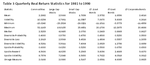
Tables 2 through 5 provide both traditional statistical moments, as well as the partial moments for six asset classes. The asset classes are commodities, large cap stocks, small cap stocks long term government bonds, intermediate term government bonds, and long term corporate bonds. Table 2 contains the statistics based on quarterly real returns for the time period 1971 to 1980. Table 3 contains the statistics for the time period 1981 to 1990, and so forth. In the periods of hyperinflation such as 1971 to 1980, commodities clearly provided superior risk adjusted performance as expressed by the omega measure. In the periods closer to the long run average, which for the forty year period was 4.41%, many other asset classes performed better than commodities. Stressful time periods such as 2001 to 2010 seem to make all investments have the same likelihood of having positive real returns. A portfolio of these investments might have led to better risk adjusted performance.
It is imprudent and dangerous for an investor to place all their capital in one asset class. We have discussed the benefits of diversification in a previous blog. The next blog looks at how a core exposure to commodities over long time periods may actually be beneficial to investors interested in protecting purchasing power.
Click To Enlarge


Table 1 Real Return Partial Moments Example


Sponsored by: EMA Softech
No comments:
Post a Comment