Blending Financial Assets and Precious Metals

By Fred Novomestky, Ph.D

In my previous blog, All That Glitters Is Not Gold, I looked at the benefits and issues of long term investments in other precious metal commodities, namely, silver and platinum. The benefits of diversification were noticeable. The platinum futures market, however, is not sufficiently large to make it accessible to investors in any meaningful manner. We found on the basis of the omega measure that the Dow Jones UBS Precious Metals Index fared somewhat better than our equal weighted portfolio of gold and silver in two time periods and worst in the other two time periods. In this blog we will see what happens when you combine precious metals with financial assets using the equally weighted portfolio.

We maintain consistency with the previous blogs by using the same four, five-year time periods of 1991 to 1995, 1996 to 2000, 2001 to 2005 and 2006 to 2010. The financial assets are large capitalization stocks, small capitalization stocks, long term government bonds, intermediate term government bonds and long term corporate bonds as computed by Ibbotson and Associates. Tables 1 to 4 contain monthly return statistics for the five asset classes, precious metals and gold futures. Gold futures were contrasted to financial assets in the blog Asset Allocation and Gold. The statistics are mean, volatility (i.e. standard deviation of returns), minimum, maximum, downside probability, downside loss downside volatility, upside probability, upside reward, upside volatility and omega measure. The upside and downside statistics are partial moments which are introduced in the blog Partial Moments – the Up and Down of Performance and Risk. Omega measure is the ratio of upside reward to downside loss.

On the basis of omega measure, most financial assets outperform precious metals and gold futures. The exception is 2006 to 2010. One has to ask if it pays to combine these commodities with financial assets. Tables 5 and 6 provide a partial answer. Table 5 presents the correlation of precious metals and financial assets while Table 6 highlights the correlations of gold with financial assets. Generally speaking, both gold and precious metals have weak positive or negative correlations with financial assets. Precious metals, as a portfolio, tend to have even more negative or weaker positive correlations. This provides an opportunity to further diversify risk.

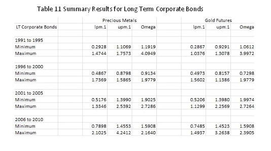
In Asset Allocation and Gold we presented omega frontier charts that show the effect of different mixes of gold and financial assets on the omega measure. These charts are not used here as they tend to have the same appearance and do not reveal information on impact of using precious metals instead of gold as a diversifying investment. Instead, we introduce a new style of analysis in Tables 7 to 11. Each table corresponds to a different financial asset. The time periods are groups of rows with Minimum and Maximum values. There are two groups of columns, one for Precious Metals and the other for Gold Futures. Each group consists of lpm.1 (downside loss), upm.1 (upside reward) and omega. Each value is associated with a portfolio of financial asset and the commodity (gold futures or precious metals). For example, the minimum and maximum upside reward for large cap stocks in Table 7 and for the time period 1991 to 1995 are 1.2799 and 1.9617 for precious metals and 0.9796 and 1.9617 for gold futures. The minimum values are the worst case outcomes for upside reward and the maximum values are the best case outcomes. Notice that precious metals had the greatest worst case outcome when compared to gold whereas both choices had the same best case outcome. In this case, an investor would prefer precious metals as a diversifying investment combined with large capitalization stocks.

If you look at best and worst case outcomes for downside loss, you would probably not want to consider blending silver with gold. The minimum values for downside loss are associated with the minimum loss portfolio as we discussed in the blog Managing Downside Loss with Gold. On the other hand, if you look at the omega measure, a risk adjusted measure of performance; the blend is clearly the best choice for almost all asset classes and time periods. I think that most investors would rather err on the side of more diversification rather than less when dabbling in commodities.


Click to Enlarge

Sponsored by: EMA Softech

All That Glitters Is Not Gold

By Fred Novomestky, Ph.D

The past several blogs have been devoted to a thoughtful analysis of the inclusion of gold along with financial assets. Using partial moments analysis, it is clear that gold exposure over longer periods of time can be reward enhancing and risk reducing. Gold is but one of several precious metals that commodity trading advisors (CTA’s) incorporate in their managed futures accounts. We take a look at two other precious metals in this blog, namely, silver and platinum.

Gold and silver play a major role in the Dow Jones UBS Commodity Index. The exposures to the various commodities in the index are reset annually. For 2011, the exposure to gold is 10.45% and the exposure to silver is 3.29%. A precious metals sub-index is computed by Dow Jones UBS for gold, silver and platinum. In addition, there is a sub-index for gold and silver. Each of these indices are based on a fully margined commodity futures contract position for the precious metals.

Let us begin by looking at return statistics for the three commodities. Table 1 summarizes the return statistics for gold, silver and platinum. We provide the traditional statistical measures for the monthly total return of these commodities as well as the upper and lower partial moments defined in our recent blog, Partial Moments – the Up and Down of Performance and Risk. We consider four, five-year time periods as we have been doing in the past several blogs, namely, 1991 to 1995, 1996 to 2000, 2001 to 2005, and 2006 to 2010. Silver has had a higher mean return when compared to gold in each of these time periods. It has also experienced more volatility than gold or platinum. Platinum has outperformed gold in three of four time periods. Using a zero return target, platinum has the highest upside probability and lowest downside probability of the three commodities.

In general, precious metal prices tend to move in comparable directions. Table 2 presents the correlations between pairs of commodities for each of the time periods. From a statistical point of view, these numbers are meaningful and substantially positive. These correlations are dynamic and change over time.

While the mean return statistics are interesting, an investor is also interested in seeing the financial rewards from investments in each of the precious metals. Figures 1 through 4 present the cumulative wealth indices for each commodity and each time period. Each curve assumes that the investor allocates 100 domestic currency units (e.g. U.S. dollars) in a commodity. At the end of each month, the entire value determined by that month’s return is reinvested for the next month. Except for 2001 to 2005, the investor would have greater wealth at the end of the five year period by an investment in silver than a similar investment in gold. Platinum is a dominant investment relative to gold except in the 2006 to 2010. With a worst case monthly return of -31.24% in 2008 along with three other significant negative months in 2008 and one in 2010, platinum underperformed both gold and silver.

The commodity trading advisor would combine multiple commodities in a managed futures account to gain the benefits of diversification. Table 3 provides comparable summary return statistics for three portfolios. The first portfolio is the Dow Jones UBS Precious Metals index which combines gold and silver with weights derived from the weights for the individual commodities from the entire index. The second portfolio equally weights gold and silver in each month of a time period. The third portfolio equally weights gold, silver and platinum in each month. Except for the 2006 to 2010 time period, the third portfolio has the highest upside probability and lowest downside probability. Equal weighted portfolios tend to outperform the Dow Jones UBS Index. Figures 5 through 8 show the cumulative wealth indices for the portfolio in each of the time periods and Table 4 summarizes the cumulative results including annualized returns and volatilities. The poor results in 2006 to 2010 for the equal weighted portfolio of three precious metals are due to the adverse performance in 2008 and 2010 for platinum highlighted above. All of these portfolios have volatilities that are normally associated with equity portfolios.

The long term investor can benefit from a strategic exposure to gold and other precious metals in their portfolio. Platinum has potentially attractive benefits. Unfortunately, open interest in the futures market is highest for gold and silver. This limits the potential for using platinum making it one of highest fruits in the market apple tree.


Click to Enlarge

Sponsored by: EMA Softech